When twitter finally released “The Algorithm” I, like many others programmers, poked around a the code base looking for things that were interesting. I’m not huge into machine learning but I am big into spatial data / GIS. So I wanted to know how Twitter is using location data and in what ways they’re using it. What I took away from my hours of trolling is that Twitter just really wants to know where you are. Twitter goes to extreme lengths to find where you are and record that information.
They use your location to know if you’re in a black listed country or if certain type of media should be restricted based to you, and they just want to recommend people to you who are near by. Among all of these different tasks one thing is common: the way that they store your location. They do so by using something called a Geohash.
Geohash definition
Before we define what a geohash is, let’s take a look at them. I’m sure we can intuit their usability just by exploration. Geohashes work by dividing the world into 32 equally sized squares. Each square is represented by a different character. Then each of these squares, are divided again into 32 rectangles each with a number or letter. So when we select another rectangle we now have two characters. And again, and again, adding a character each time. Notice how we can see the selected characters being recorded up at the top here. Each time we select another rectangle the number of characters grows and the size of the box shrinks. This happens up to 12 times.
That’s right, geohashes pretend the earth is flat. One point for the flat earthers. The earth is actually round and that’s why S2 is better.
The characters that we have recorded correspond to a rectangle somewhere on the earth. The number of characters refers to the precision of the geohash. Said a different way, the more characters we have in our geohash the more accurate the measurement.
When we get down to 12 character we are working with a rectangle that is literally millimeters wide. That’s precise enough for just about every single use case I can think of. There is a technical reason why geohashes are limited to 12 characters that we will get into later.
Spatial Indexing
Say we have a longitude and latitude. This coordinate represents some place on earth. We can then encode that location into a string of numbers and letters up to 12 characters long. These twelve character characters? That is all that a geohash is. It is a way to represent a region on the earth using a single value.
Spatial indexes are a collection of algorithms or tools that make it easier to represent locations on the earth without having to use coordinates. You might be familiar with a few of them such as uber’s H3 Hexagonal spatial index or Google’s S2 index for spherical geometry. If you’re an R user and you’ve used the package {sf} you’ve already used S2 whether you know it or not.
Geohash properties
Geohashes have a number of properties that make them rather handy to work with. The most important of which is that the closer to points are, they will have an increasing number of shared characters in their geohash. The number of shared letters from the beginning of the geohash to the end can give you a really good estimate of proximity!
This is super useful particularly for databases. Databases are good at querying strings. They are not so good at calculating pairwise distance matrix for every single location in your database–imagine how many values that would be! If you wanted to find locations within some distance of a point you it would be far more efficient to search based on the geohash. Based on the approximate distance you can truncate geohashes to say, 6 characters, to find locations within 3/4ths of a mile. Any locations that share the first 6 characters of a geohash will be, at most, 0.75 miles away (as the crow flies, that is).
Boston example
Let’s look at an example. You’re a tourist in Boston and you’ve just gotten off the train at Park Street station and you want a coffee. You don’t want a Dunkin’ or a coffee from the weird McDonalds across the street. You want to spend $6 dollars on a well made espresso. I just so happen to know that there is a phenomenal cafe called George Howell a stones throw away. Let’s look at some code that could do this search and ranking for us.
First, lets take a look at the geohash 6 around Park Street. Anything that falls into this grid would be a reasonable location to return. Now, let’s look at some code.
If you don’t know R, that’s okay. The code is straight forward and I want you to take away the use case not the code.
First, we store the location of Park Street station and then encode it as a geohash.
The following objects are masked from 'package:stats':

    filter, lag
The following objects are masked from 'package:base':

    intersect, setdiff, setequal, union
library(geohashTools)library(populartimes)# store park street coordinatespark_street_loc<-c(42.35675660592967, -71.06224330327713)# encode the geohashpark_street<-gh_encode(park_street_loc[1], park_street_loc[2], 12)park_street
[1] "drt2yyy1cxwy"
Next, using the location we can query Google Maps looking for cafes using the Park Street coordinates.
res<-text_search( location =park_street_loc, query ="espresso", type ="cafe")res[c("name", "rating", "price_level")]
Now we need to validate how close each of these places are to Park Street. We could of course do this by calculating the distance between each coordinate and Park Street. But that is overall computationally intensive. We can instead limit our result based on the number of shared characters in the geohash.
With the help of the extendr discord we have a function that can count the number of sequential characters. There’s a good blog post on this topic here.
Using this function we can count the number of shared characters for each location and remove any places that don’t have at least 6 shared characters.
In this code chunk we first create a column to store the geohash. Then we count the number of shared characters to the Park Street geohash, filter() to 6 or more shared characters, and then print the data nicely.
Once limited, the option is clear as day. The closest and best coffee shop is George Howell. I hope you appreciate through this simple example how power it storing a location as a string can be.
This is unfortunately about the most that you’ll take away from most videos on geohashes. But we’re just getting started. To me this is insufficient. Sure, you may now know how to use a geohash. My goal here is to have you walk away understanding how geohashes work. That’s an important distinction.
So if you’re ready, we’re going to go into a very deep dive. We’re going to spend the rest of this time walking through the geohash algorithm step by step in such a way thay you will be able to implement it yourself afterwards.
History
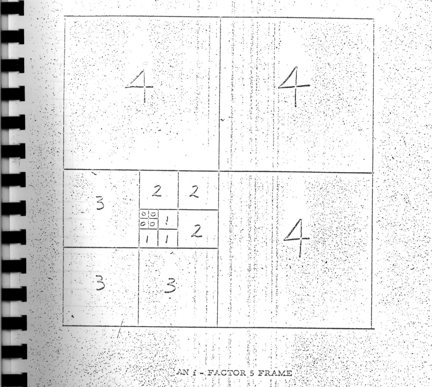
The algorithm that we just used was reinvented in 2008 by a fella named Gustavo Niemeyer. I say reinvented because back in the 60s another fella name G.M. Morton from IBM wrote this paper “A Computer Oriented Geodetic Database and a New Technique in File Sequencing.”
Which looks quite a lot like a geohash with its recursive gridding.
What is funny is that Gustavo Niemeyer claims to have not known about this prior work–which I do not doubt. It is not the first time in history that the same thing has been discovered by two separate people in tow separate points in time. Somewhat like how we now have Liebnitz and Newton notation for derivatives.
Unfortunatey for GM Morton, it is Gustavo’s version that we all use.
https://en.wikipedia.org/wiki/Geohash
Z-order curves
At the root, a geohash is an implementation of a Z-order curve. It’s not necessary to understand Z-order curves in all of of their intricacies to truly understand geohashes but its worth diving into a bit. Shoot, I don’t even fully get them.
In the field of mathematical analysis there is an entire subfield dedicated to what are called “space filling curves.” In essence, they are a suite of algorithms that map 2 or 3 dimensional data into a single dimension. The Z-order curve is one of these space filling curves that is used to map 2 dimensional data into one dimension. The Z-order curve is used a bunch in big data technologies like Apache Spark, Cassandra, and Parquet to speed up search.
But there is no way I can do justice to explaining them so I really recommend that you watch this 3blue1brown video on them.
In geography we are always dealing in at least 2 dimensions: longitude and latitude. Using a Z-order curve we can encode longitude and latitude as a single value and that’s exactly what geohash does. But how?
Now pay attention here. This is the only important part about a z-order curve I want you to care about. We are going to create a z-coordinate. A z-coordinate maps an x and a y dimension to a single z dimension–this z-coordinate is what a geohash is.
Say we have two numbers x and y. x is equal to 23 and y is equal to 42. From x and y we can create a third value, z (hence the name).
Z-coordinates
I’m about to make a leap here. Stay with me. Both of these numbers can be represented in binary as a combination of 0’s and 1s. In binary, 23 is 00010111 and 42 is 00101010. Each number is represented by 8 different 0s or 1s so they are 8 bit numbers—integers, to be exact. To get our z-coordinate all we need to do is “interleave” them.
Interleaving sounds fancy but it’s super simple. I like to think of interleaving as weaving two leavings together by alternating one and another. Our z-coordinate is the sequence of bits that results from interleaving x and y.
To do this, we take the first value of x followed by the first value of y. Then we append the second value of x followed by the second value of y. We do this until we’ve exhausted all bits in x and y.
The result is a sequence of 16 bits 0000011001101110. Instead of having 8 bits, we now have 16 bits. Or a 16 bit integer. This is an important detail, when we interleave two numbers we always double the number of bits used.
that interleaving of bits is all that a geohash really is.
So do we just convert our x and y values to binary and then interleave them? Well, no. Of course it’s not that simple. There are two ah hahs! The first has to do with the limitations of modern computing.
Back to bits.
In R, and python, and most other systems, numbers that contain values after the decimal place are known as “double precision floating points” which is a really long way of saying they are 64 bit numbers. Again, that means that our numbers are represented by 64 sequential 1s or 0s.
When we interleave two floats we will end up with a 128 bit number. That’s a bit more than most languages and tools are able to handle. Though that’s going to change in the next few years I bet.
Since we can only handle 64 bits, we have to truncate x and y to 32 bits so that when we interleave the two we end up with 64 bits.
The geohash algorithm implements a pretty creative way of representing numbers as binary. The binary representation is actually a way of specifying the location on the number line.
Start with an X value. X can fall anywhere in the interval [-180, 180). We break that interval into two in the middle that is left inclusive. If the value falls in the left interval then it gets the value of 0. If it falls in the right interval, then it gets the value of 1. We can do this up to 32 times–remember, 32 bits!
For the value 19 it falls into the right interval so the first bit is the value of 1. Now we set our initial interval to [0, 180). We again partition it in the middle into 2 intervals. Since 19 falls in the left interval it gets the value of 0. So on an so forth until we do this 32 times!
We do the same thing for latitude but the initial bounds are different. They are [-90, 90). Again, repeat this 32 times.
We can look at what this might look like on the plane.
We start with a point that is in the upper left quadrant. We partition on our longitude. Since it’s in the right interval it gets the value 1. Now we partition it again. It’s in the left, it gets the value of 0. Again we partition. It is in the right. It gets the value of 1. One last time we partiion. It falls into the right interval so it gets the value of 1.
Once we have completed our encoding on longitude we can begin encoding our latitude. The point falls in the right interval which, when viewed on the plane, is actually the top one. And again, its in the top. So far we have the bits 1 and 1. Then again. This time it is on the bottom. It get’s a 0. The last time it is at the top and gets a 1.
When we interleave the results of our encoding we get the value of 1 1 0 1 1 0 1 1.
Converting from binary to geohash
I told you that a geohash is just a z-coordinate. But now we have a binary z-coordinate and it looks nothing like the geohashes I showed you earlier. Well, there’s one last step that we have to take to go from our binary z-coordinate to a geohash.
Geohashes are “base32” encoded. What does that mean?
The number system that we use and are familiar with is called base 10. That’s because we have 10 unique digits that we use to represent values 0-9.
Binary is a base 2 number system because it uses the two digits 0 and 1 to represent values.
The n refers to how many character are in the alphabet being used to represent values.
So base 32 means that there are 32 digits that are used to represent values. These are a combination of letters and numbers. Typically, these are the letters A through Z and the numbers 2 through 7.
Though the Geohash algorithm has it’s own base 32 alphabet called the “geohash alphabet” (wiki source). It contains the numbers 0 through 9 and the entire alphabet except a, i, l, and o because they look similar to numbers (except a)—they just needed 1 fewer character.
To utilze the alphabet we need to define a lookup table that has our characters by position.
Base 32 encoding
Base 32 requires 5 bits to represent each character. Having 5 bits gives us 32 possible possible combinations. From 00000 being 0 in binary and 11111 being 31 in binary.
You can think of this as 2 * 2 * 2 * 2 * 2 possibilities or 2^5.
Take this series of bits.
We can begin to decode it by first breaking it up into sequences of 5 bits.
For each of these 5 bits we figure out what number they represent in our decimal system.
So our first chunk of 5 bits is 11010. That is equal to 26. Our second group of 5 bits is equal to 2. Then 20, 14, 9, and 0.
Now instead of a series of 5 bits we have a number between 0 and 31 inclusive. We take these numbers and go back to our alphabet looking up each one by position. We look up the 26th element (this example uses rust so its base 0) and the look up returns u. We do the same for the 2nd element and get 2. We do this for all of our digits and end up with the the characters u 2 n f 9 0. Boom. That is our geohash!
Once we have encode each of our 5 bits from numbers into base 32 we concatenate them and we have our geohash!
Next we’re going to look at how we can do this in code. But first let’s recap everything up until now.
Recap
A geohash is a one dimensional encoding from 2 dimensions. We create a Z coordinate from an x and y coordinate. To create the z coord we need to encode our x and y as binary. We do through a sequence of partitions along the number line. We split our range in half to create two intervals. If the value falls into the right interval we record a 1. If it is the left interval we record a 0. We then adjust our interval to be half of which one the point fell in and we repeat until we get 32 bits for both values.
Once you have encoded both x and y. We need to interleave them to create a new sequence of 64 total bits.
After which we break the bits into groups of 5 bits. Once the bits have been broken up we translate them into integers.
From there, we encode them into our base 32 alphabet by looking up based on position.
Coding it
For this example I was torn between using Rust or R for the example. If you have a preference one way or the other, please let me know in the comments.
The first thing that we need to do is define our x and y values or our coordinate.
Next we need to specify the precision of our geohash. For our first example let’s look at the full 12 digits. So lets set precision equal to 12.
Then let’s instantiate two vectors that we will us to search along the x and y axis to encode our values into binary. Each vector will have three elements to represent our two intervals. It will have a lower value, a mid point, and an upper bound.
Next we need to pre-allocate the vectors which will store our the binary encoding or our x and y values. We encode only 32 bits for x and y because we’re limited to 64 bits in floating point numbers.
Next, we need to begin to encode our x and y values. The simplest way to do this is through a for loop.
Since we
notes
Medium post that helped me get to the last part https://yatmanwong.medium.com/geohash-implementation-explained-2ed9627a61ff Factual blog post http://web.archive.org/web/20220620005549/https://www.factual.com/blog/how-geohashes-work/